Parameter Learning for simple PDE
In this tutorial we will learn how to learn a parameter of a PDE using gradient descent in Physika. We will use the 1D heat equation as our example — a parabolic partial differential equation first developed by Joseph Fourier in 1822 to model how heat diffuses through a given region.
The Equation
The 1D heat equation is:
Where \(u\) is temperature, \(x\) is space, \(t\) is time, and \(\alpha\) is the thermal diffusivity parameter we want to learn.
Helper functions
def get_1d_array_length(x: ℝ[m]): ℝ:
    total: ℝ = 0
    temp: ℝ = 0
    for i:
        temp = x[i]
        total += 1
    return total

def zero_1d_array(len: ℝ): ℝ[m]:
    results: ℝ[len] = for i: ℕ(len) -> i*0
    return results

def linspace(start: ℝ, end: ℝ, n: ℕ): ℝ[n]:
    x: ℝ[n] = zero_1d_array(n)
    dx: ℝ = (end - start) / (n - 1)
    for i:ℕ(0, n):
        x[i] = start + i * dx
    return x
Step 1: Discretize the PDE
We discretize the spatial derivative using finite differences:
In Physika:
def heat_equation(T: ℝ[m], dx: ℝ, α: ℝ): ℝ[m]:
    nx: ℝ = get_1d_array_length(T)
    f: ℝ[m] = zero_1d_array(nx)
    for i:ℕ(1, nx-1):
        f[i] = α / dx ** 2 * (T[i-1] - 2*T[i] + T[i+1])
    return f
heat_equation computes the right hand side of the PDE at every interior
grid point, returning the rate of change of temperature.
Step 2: Build the Solver
We integrate the PDE forward in time using Forward Euler, with Dirichlet boundary conditions (zero temperature at both ends):
def solver(α:ℝ, T0: ℝ[m], dx: ℝ, dt:ℝ, nt: ℝ): ℝ[m]:
    T: ℝ[m] = T0
    last_index: ℝ = get_1d_array_length(T)
    for i:ℕ(0, nt):
        T = T + dt * heat_equation(T, dx, α)
        T[0] = 0
        T[last_index-1] = 0
    return T
Note
The time step dt must satisfy the CFL stability condition:
We use a Fourier number of 0.49 to stay just below this limit.
Step 3: Set Up the Grid
We create a uniform spatial grid over \([0, 1]\) with 21 points:
lx: ℝ = 1.0
nx: ℝ = 21
dx: ℝ = lx / (nx - 1)
x: ℝ[nx] = linspace(0, lx, nx)
Step 4: Generate Ground Truth Data
We pick a Gaussian initial condition centered at \(x = 0.5\) and run the solver with the true thermal diffusivity \(\alpha = 0.4\):
true_alpha: ℝ = 0.4
fourier: ℝ = 0.49
dt: ℝ = fourier * dx**2 / true_alpha
nt: ℝ = 100

T0: ℝ[nx] = zero_1d_array(nx)
for i:ℕ(0, nx):
    T0[i] = exp(-50 * (x[i] -0.5)**2)

true_values: ℝ[m] = solver(true_alpha, T0, dx, dt, nt)
The Gaussian pulse will diffuse outward over time — the rate of diffusion is controlled by \(\alpha\).
Step 5: Define the Loss
We measure the mean squared error between predicted and true final temperature profiles:
def calculate_loss(α: ℝ): ℝ:
    predictions: R[m] = solver(α, T0, dx, dt, nt)
    loss: ℝ = 0.0
    for i:ℕ(0, nx):
        diff = predictions[i] - true_values[i]
        loss += diff ** 2
    return loss / nx
Step 6: Train with Gradient Descent
We start with an initial guess of \(\alpha = 0.1\) and run 500 epochs of gradient descent:
α: ℝ = 0.1
learning_rate: ℝ = 0.1
epochs: ℕ = 500

for i:ℕ(epochs):
    g = grad(calculate_loss, α)
    α = α - learning_rate * g
Physika differentiates through the entire PDE solver automatically — including the time loop and finite difference stencil.
Step 7: Visualize Results
pred_values: ℝ[m] = solver(α, T0, dx, dt, nt)
plot_trajectories(true_values, pred_values)
After 500 epochs, alpha should be close to 0.4 and the predicted
temperature profile should match the true one.
Note
plot_trajectories is not a built-in Physika function. To use it,
add the following helper to physika/runtime.py:
def plot_trajectories(true_values, pred_values):
      import matplotlib.pyplot as plt

      plt.plot(true_values.detach().numpy(), label="True")
      plt.plot(pred_values.detach().numpy(), '--', label="Predicted")

      plt.xlabel("x")
      plt.ylabel("Temperature")
      plt.title("True vs Predicted Solution (Final Time)")
      plt.legend()
      plt.show()
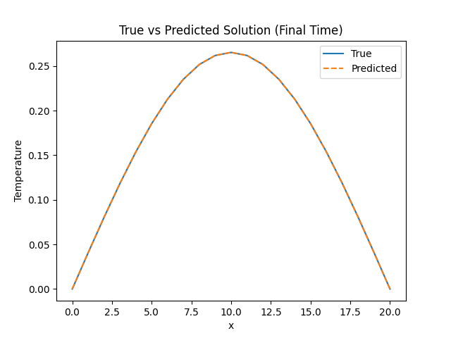
Comparison between ground truth and learned trajectory after training.
Full Code
def get_1d_array_length(x: ℝ[m]): ℝ:
    total: ℝ = 0
    temp: ℝ = 0
    for i:
        temp = x[i]
        total += 1
    return total

def zero_1d_array(len: ℝ): ℝ[m]:
    results: ℝ[len] = for i: ℕ(len) -> i*0
    return results

def linspace(start: ℝ, end: ℝ, n: ℕ): ℝ[n]:
    x: ℝ[n] = zero_1d_array(n)
    dx: ℝ = (end - start) / (n - 1)
    for i:ℕ(0, n):
        x[i] = start + i * dx
    return x

def heat_equation(T: ℝ[m], dx: ℝ, α: ℝ): ℝ[m]:
    nx: ℝ = get_1d_array_length(T)
    f: ℝ[m] = zero_1d_array(nx)
    for i:ℕ(1, nx-1):
        f[i] = α / dx ** 2 * (T[i-1] - 2*T[i] + T[i+1])
    return f

def solver(α:ℝ, T0: ℝ[m], dx: ℝ, dt:ℝ, nt: ℝ): ℝ[m]:
    T: ℝ[m] = T0
    last_index: ℝ = get_1d_array_length(T)
    for i:ℕ(0, nt):
        T = T + dt * heat_equation(T, dx, α)
    T[0] = 0
    T[last_index-1] = 0
    return T

lx: ℝ = 1.0
nx: ℝ = 21
dx: ℝ = lx / (nx - 1)
x: ℝ[nx] = linspace(0, lx, nx)

true_alpha: ℝ = 0.4
fourier: ℝ = 0.49
dt: ℝ = fourier * dx**2 / true_alpha
nt: ℝ = 100

T0: ℝ[nx] = zero_1d_array(nx)
for i:ℕ(0, nx):
    T0[i] = exp(-50 * (x[i] -0.5)**2)

true_values: ℝ[m] = solver(true_alpha, T0, dx, dt, nt)

def calculate_loss(α: ℝ): ℝ:
    predictions: R[m] = solver(α, T0, dx, dt, nt)
    loss: ℝ = 0.0
    for i:ℕ(0, nx):
        diff = predictions[i] - true_values[i]
        loss += diff ** 2
    return loss / nx

α: ℝ = 0.1
learning_rate: ℝ = 0.1
epochs: ℕ = 500

for i:ℕ(epochs):
    g = grad(calculate_loss, α)
    α = α - learning_rate * g

pred_values: ℝ[m] = solver(α, T0, dx, dt, nt)
plot_trajectories(true_values, pred_values)