Parameter Learning of 1D wave equation

In this tutorial we will learn how to estimate/learn parameter of 1D wave equation using gradient descent in Physika. The 1D wave equation describes how a wave propagates through a medium — examples include sound waves travelling through air, seismic waves propagating through the earth, and vibrations along a guitar string.

Given observed wave data, our goal is to find the value of \(c\) that makes our simulation match it. This is called parameter learning. Gradient descent does this by repeatedly computing how the error changes with respect to \(c\) and updating it in the direction that reduces the error.

The Equation

The 1D wave equation is:

\[\begin{align*} \frac{\partial^2 u}{\partial t^2} &= c^2 \frac{\partial^2 u}{\partial x^2} \end{align*}\]

where \(u(x, t)\) is the displacement, \(x\) is space, \(t\) is time, and \(c\) is the wave speed, the parameter we want to learn.

Helper functions

def get_1d_array_length(x: ℝ[m]): ℝ:
    total: ℝ = 0
    temp: ℝ = 0
    for i:
        temp = x[i]
        total += 1
    return total

def zero_1d_array(len: ℝ): ℝ[m]:
    results: ℝ[len] = for i: ℕ(len) -> i*0
    return results

def linspace(start: ℝ, end: ℝ, n: ℕ): ℝ[n]:
    x: ℝ[n] = zero_1d_array(n)
    dx: ℝ = (end - start) / (n - 1)
    for i:ℕ(0, n):
        x[i] = start + i * dx
    return x

Step 1: Discretize the PDE

We approximate the second spatial derivative using centered finite differences:

\[\begin{align*} \frac{\partial^2 u}{\partial x^2} \approx \frac{u_{i-1} - 2u_i + u_{i+1}}{\Delta x^2} \end{align*}\]

def wave_equation(u: ℝ[m], dx: ℝ, c: ℝ): ℝ[m]:
    nx: ℕ = get_1d_array_length(u)
    f: ℝ[m] = zero_1d_array(nx)
    for i:ℕ(1, nx-1):
        f[i] = (c**2 / dx**2) * (u[i-1] - 2*u[i] + u[i+1])
    return f

The boundary points are left as zero, enforcing Dirichlet boundary conditions \(u(0, t) = u(1, t) = 0\).

Step 2: Build the solver

Because the wave equation is second order in time, the solver must track two states at each step — the previous displacement u_prev and the current displacement u_curr.

We start with the wave equation:

\[\begin{align*} \frac{\partial^2 u}{\partial t^2} &= c^2 \frac{\partial^2 u}{\partial x^2} \end{align*}\]

Approximating the second time derivative with centered finite differences:

\[\begin{align*} \frac{\partial^2 u}{\partial t^2} &\approx \frac{u_i^{n+1} - 2u_i^n + u_i^{n-1}}{\Delta t^2} \end{align*}\]

Approximating the second space derivative with centered finite differences:

\[\begin{align*} \frac{\partial^2 u}{\partial x^2} &\approx \frac{u_{i-1}^n - 2u_i^n + u_{i+1}^n}{\Delta x^2} \end{align*}\]

Substituting both into the wave equation and rearranging for \(u_i^{n+1}\):

\[\begin{align*} \frac{u_i^{n+1} - 2u_i^n + u_i^{n-1}}{\Delta t^2} &= c^2 \frac{u_{i-1}^n - 2u_i^n + u_{i+1}^n}{\Delta x^2} \end{align*}\]

\[\begin{align*} u_i^{n+1} &= 2u_i^n - u_i^{n-1} + \Delta t^2 \cdot \frac{c^2}{\Delta x^2} \left( u_{i-1}^n - 2u_i^n + u_{i+1}^n \right) \end{align*}\]

def solver(c: ℝ, u0: ℝ[m], dx: ℝ, dt: ℝ, nt: ℝ): ℝ[m]:
    u_prev: ℝ[m] = u0
    u_curr: ℝ[m] = u0
    nx: ℕ = get_1d_array_length(u0)
    for n:ℕ(0, nt):
        accel = wave_equation(u_curr, dx, c)
        u_next = 2*u_curr - u_prev + dt**2 * accel
        u_next[0] = 0
        u_next[nx-1] = 0
        u_prev = u_curr
        u_curr = u_next
    return u_curr

Step 3: Set Up the Grid

We discretize the spatial domain \([0, 1]\) into nx points and the time domain \([1, 2]\) into nt steps, giving uniform spacings \(\Delta x\) and \(\Delta t\):

nx: ℝ = 30
nt: ℝ = 30

a: ℝ = 0
b: ℝ = 1
t0: ℝ = 0
tf: ℝ = 1

dx: ℝ = (b-a)/(nx-1)
dt: ℝ = (tf-t0)/(nt-1)

Step 4: Generate Ground Truth Data

We fix the true wave speed at \(c = 0.5\) and set the initial condition to a sine wave:

\[\begin{align*} u(x, 0) &= \sin(2\pi x) \end{align*}\]

Running the solver with this initial condition and the true parameter produces the ground truth trajectory that we will try to recover:

pi: ℝ = 3.14
true_c: ℝ = 0.5

x: R[m] = linspace(a, b, nx)
u0: ℝ[nx] = zero_1d_array(nx)
for i:ℕ(0, nx):
    u0[i] = sin(2 * pi * x[i])


true_values: R[m] = solver(true_c, u0, dx, dt, nt)

Step 5: Define the Loss

The loss function measures the mean squared error between the predicted final state and the true final state:

\[\begin{align*} \mathcal{L}(c) &= \frac{1}{N} \sum_{i=0}^{N - 1} \left( u_i^{\text{pred}} - u_i^{\text{true}} \right)^2 \end{align*}\]

def calculate_loss(c: ℝ): ℝ:
    predictions: R[m] = solver(c, u0, dx, dt, nt)
    loss: ℝ = 0.0
    for i:ℕ(0, nx):
        diff = predictions[i] - true_values[i]
        loss += diff ** 2
    return loss / nx

Step 6: Train with Gradient Descent

We start with an initial guess of c = 0.1 and run 200 epochs of gradient descent:

c: ℝ = 0.1
learning_rate: ℝ = 0.01
epochs: ℕ = 200

for i:ℕ(epochs):
    physika_print(i)
    g = grad(calculate_loss, c)
    c = c - learning_rate * g

Physika differentiates through the entire PDE solver automatically — including the time loop and finite difference stencil.

Step 7: Visualize Results

pred_values: ℝ[m] = solver(c, u0, dx, dt, nt)
plot_trajectories(true_values, pred_values)

After 200 epochs, c should be close to 0.5.

Note

plot_trajectories is not a built-in Physika function. To use it, add the following helper to physika/runtime.py:

def plot_trajectories(true_values, pred_values):
      import matplotlib.pyplot as plt

      plt.plot(true_values.detach().numpy(), label="True")
      plt.plot(pred_values.detach().numpy(), '--', label="Predicted")

      plt.xlabel("x")
      plt.ylabel("u(x, tf)")
      plt.title("True vs Predicted Solution (Final Time)")
      plt.legend()
      plt.show()

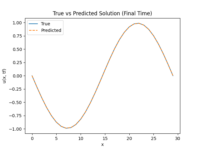
Learned PDE trajectory vs ground truth — Comparison between ground truth and learned trajectory after training.

Full Code

def get_1d_array_length(x: ℝ[m]): ℝ:
    total: ℝ = 0
    temp: ℝ = 0
    for i:
        temp = x[i]
        total += 1
    return total

def zero_1d_array(len: ℝ): ℝ[m]:
    results: ℝ[len] = for i: ℕ(len) -> i*0
    return results

def linspace(start: ℝ, end: ℝ, n: ℕ): ℝ[n]:
    x: ℝ[n] = zero_1d_array(n)
    dx: ℝ = (end - start) / (n - 1)
    for i:ℕ(0, n):
        x[i] = start + i * dx
    return x

def wave_equation(u: ℝ[m], dx: ℝ, c: ℝ): ℝ[m]:
    nx: ℕ = get_1d_array_length(u)
    f: ℝ[m] = zero_1d_array(nx)
    for i:ℕ(1, nx-1):
        f[i] = (c**2 / dx**2) * (u[i-1] - 2*u[i] + u[i+1])
    return f

def solver(c: ℝ, u0: ℝ[m], dx: ℝ, dt: ℝ, nt: ℝ): ℝ[m]:
    u_prev: ℝ[m] = u0
    u_curr: ℝ[m] = u0
    nx: ℕ = get_1d_array_length(u0)
    for n:ℕ(0, nt):
        accel = wave_equation(u_curr, dx, c)
        u_next = 2*u_curr - u_prev + dt**2 * accel
        u_next[0] = 0
        u_next[nx-1] = 0
        u_prev = u_curr
        u_curr = u_next
    return u_curr

nx: ℝ = 30
nt: ℝ = 30

a: ℝ = 0
b: ℝ = 1
t0: ℝ = 0
tf: ℝ = 1

dx: ℝ = (b-a)/(nx-1)
dt: ℝ = (tf-t0)/(nt-1)


pi: ℝ = 3.14
true_c: ℝ = 0.5

x: R[m] = linspace(a, b, nx)
u0: ℝ[nx] = zero_1d_array(nx)
for i:ℕ(0, nx):
    u0[i] = sin(2 * pi * x[i])


true_values: R[m] = solver(true_c, u0, dx, dt, nt)


def calculate_loss(c: ℝ): ℝ:
    predictions: R[m] = solver(c, u0, dx, dt, nt)
    loss: ℝ = 0.0
    for i:ℕ(0, nx):
        diff = predictions[i] - true_values[i]
        loss += diff ** 2
    return loss / nx


c: ℝ = 0.1
learning_rate: ℝ = 0.01
epochs: ℕ = 200

for i:ℕ(epochs):
    physika_print(i)
    g = grad(calculate_loss, c)
    c = c - learning_rate * g

pred_values: ℝ[m] = solver(c, u0, dx, dt, nt)
plot_trajectories(true_values, pred_values)