Convolutional Neural Networks
In this tutorial we implemented Convolutional Neural networks in physika and trained it on simple classification task with MNIST dataset.
Dataset
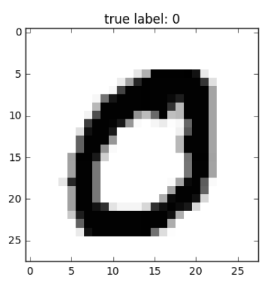
We trained CNN model on simple MNIST dataset for classifications task, for 10 classes numbers ranging from 0 to 10
dataset = create_dataset(80, 100)
train_dataset = dataset[0]
test_dataset = dataset[1]

train_X = train_dataset[0]
train_y = train_dataset[1]
test_X = test_dataset[0]
test_y = test_dataset[1]
Note
create_dataset is not a built-in Physika function. To use it,
add the following helper to physika/runtime.py:
def create_dataset(train_test_split = 80, total_dataset_size = 40):
    import torch
    from torchvision import datasets, transforms

    transform = transforms.ToTensor()

    mnist = datasets.MNIST(
        root="./data",
        train=True,
        download=True,
        transform=transform
    )

    X = []
    y = []

    # take first total_dataset_size samples
    for i in range(total_dataset_size):
        image, label = mnist[i]

        # [1,28,28] -> [28,28]
        image = image.squeeze(0)
        X.append(image)
        y.append(label)
    X = torch.stack(X)
    y = torch.tensor(y)

    # split index
    split_index = int(
        (train_test_split / 100.0)
        *
        total_dataset_size
    )

    # train split
    X_train = X[:split_index]
    y_train = y[:split_index]

    # test split
    X_test = X[split_index:]
    y_test = y[split_index:]
    train_data = [X_train, y_train]
    test_data = [X_test, y_test]
    return [train_data, test_data]
Each input or each single digit is size of 1x28x28, 1 is single channel image of grayscale and 28x28 is Height and width
Helper functions
def get_1d_array_length(x: ℝ[m]): ℝ:
    total: ℝ = 0
    temp: ℝ = 0
    for i:
        temp = x[i]
        total += 1
    return total

def get_2d_array_num_rows(x: ℝ[m, n]): ℝ:
    total: ℝ = 0
    temp: ℝ = 0
    for i:
        temp = x[i]
        total += 1
    return total

def zero_1d_array(len: ℝ): ℝ[m]:
    results: ℝ[len] = for i: ℕ(len) -> i*0
    return results

def zero_2d_array(rows: ℝ, cols: ℝ): ℝ[m, n]:
    results: ℝ[rows, cols] = for i:ℕ(rows) -> for j:N(cols) -> j*0
    return results

def get_sum_of_1d_array(x: ℝ[m]): ℝ:
    total = 0
    for i:
        total += x[i]
    return total

def max(x: ℝ, y: ℝ): ℝ:
    if x>y:
        return x
    else:
        return y
Activation functions
After the convolution operation produces an output feature map, we apply the ReLU activation function element-wise to every value.
ReLU helps the model learn non-linear patterns by removing negative values.
Mathematically, ReLU is defined as:
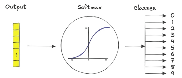
In the final layer of a convolutional neural network, the model produces raw output scores known as logits. We apply the softmax function to convert these logits into a probability distribution over the output classes. Mathematically:
def relu(x: ℝ): ℝ:
    if x>0:
        return x
    else:
        return 0.0

def relu2d(x: ℝ[H, W]): ℝ[H, W]:
    rows: ℝ = get_2d_array_num_rows(x)
    cols: ℝ = get_1d_array_length(x[0])
    results: ℝ[rows, cols] = zero_2d_array(rows, cols)
    for i:ℕ(rows):
        for j:ℕ(cols):
            results[i, j] = relu(x[i, j])
    return results

def softmax(x: ℝ[m]): ℝ[m]:
    len_x: ℝ = get_1d_array_length(x)
    exps_array: ℝ[m] = for i:ℕ(len_x) -> exp(x[i])
    total: ℝ = get_sum_of_1d_array(exps_array)
    results: ℝ[len_x] = for i:ℕ(len_x) -> exps_array[i] / total
    return results
ConvNet class
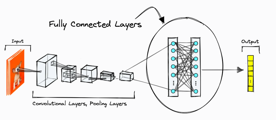
Lets bulid the full convnets class step by step. The overall architecture of our network (forward pass) follows the pipeline:
Convolution -> ReLU -> MaxPool -> Flatten -> Linear -> Softmax
We will implement this each block in separate functions
1. Convolution block
The convolution layer is the core building block of a convolutional neural network.
It expects:
an input image or feature map (shape :- 28x28 for this dataset)
a convolution kernel
a bias term
Mathematically, the layer slides the kernel across the input tensor and computes local weighted sums at every spatial location.
The input tensor is defined as:
The convolution kernel is defined as:
The layer produces a new feature map containing extracted spatial features such as:
edges
textures
local patterns
The output spatial dimensions are computed using:
where:
\(H, W\) are the input dimensions
\(K\) is the kernel size
\(P\) is the padding
\(S\) is the stride
The output feature map is therefore:
Here we assume padding as 1 and stride as 1
def conv2d(input: ℝ[H, W], kernel: ℝ[K, K], bias: ℝ): ℝ[m, n]:
    out_H: ℝ = get_2d_array_num_rows(input) - get_2d_array_num_rows(kernel) + 1
    out_W: ℝ = get_1d_array_length(input[0]) - get_1d_array_length(kernel[0]) + 1
    results: ℝ[out_H, out_W] = zero_2d_array(out_H, out_W)
    for i:ℕ(out_H):
        for j:ℕ(out_W):
            acc = 0
            for ki:ℕ(len(kernel)):
                for kj:ℕ(len(kernel[0])):
                    acc += input[i+ki, j+kj] * kernel[ki, kj]
            results[i, j] = acc + bias
    return results
2. Max Pooling Block
The max pooling layer reduces the spatial dimensions of the feature map while preserving the most important activations.
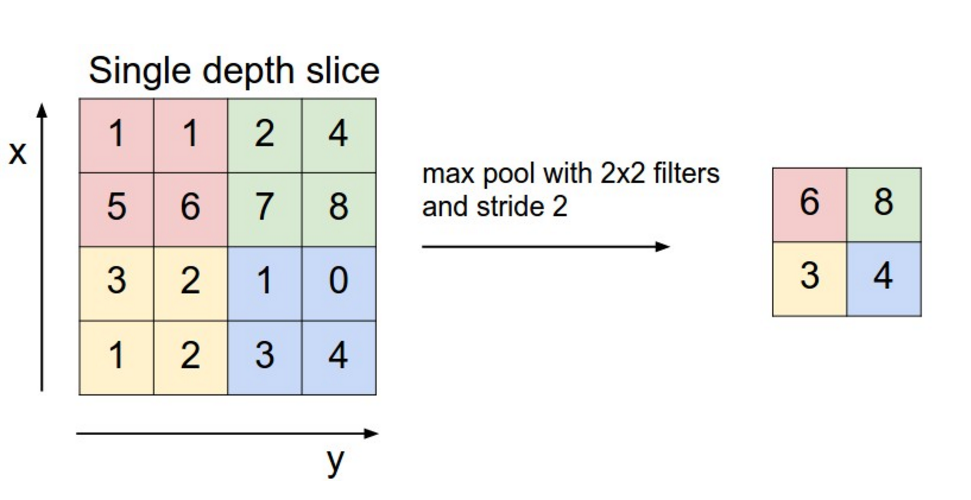
The output spatial dimensions are computed using:
where:
\(K\) is the pooling window size
\(S\) is the stride
def maxpool2d(x: ℝ[m, n]): ℝ[m, n]:
    stride: ℝ = 2
    rows: ℝ = get_2d_array_num_rows(x) / 2
    cols: ℝ = get_1d_array_length(x[0]) / 2
    results: ℝ[rows, cols] = zero_2d_array(rows, cols)
    for i:ℕ(rows):
        for j:ℕ(cols):
            a = x[i*stride, j*stride]
            b = x[i*stride, j*stride + 1]
            c = x[i*2+1, j*2]
            d = x[i*2+1, j*2+1]
            results[i, j] = max(a, max(b, max(c, d)))
    return results
Flatten Block
The flatten layer converts a 2D feature map into a 1D vector so that it can be fed into the linear classification layer.
The input tensor is defined as:
The flattened vector length is computed as:
The output tensor therefore becomes:
The flatten operation maps every spatial coordinate:
into a 1D index:
Visualization of Convolution block + pooling block + neural network
def flatten(x: ℝ[m, n]): ℝ[n]:
    rows: ℝ = get_2d_array_num_rows(x)
    cols: ℝ = get_1d_array_length(x[0])
    new_len: ℝ = rows*cols
    results: ℝ[new_len] = zero_1d_array(new_len)
    for i:ℕ(rows):
        for j:ℕ(cols):
            results[i*cols + j] = x[i, j]
    return results
def linear(x: ℝ[n], weight: ℝ[m, n], bias: ℝ[m]): ℝ[m]:
    out: ℝ = get_1d_array_length(bias)
    inp: ℝ = get_1d_array_length(x)
    results: ℝ[out] = zero_1d_array(out)
    for i:ℕ(out):
        acc = 0
        for j:ℕ(inp):
            acc += weight[i, j] * x[j]
        results[i] = acc + bias[i]
    return results
Forward Pass
The forward pass defines how data flows through the complete convolutional neural network.
Convolution -> ReLU -> MaxPool -> Flatten -> Linear -> Softmax
The Physika implementation is:
def λ(input: ℝ[H, W]) -> ℝ[m]:
    conv1: ℝ[m, n] = this.conv2d(input, this.kernel, this.b1)
    relu1: ℝ[H, W] = relu2d(conv1)
    pool1: ℝ[m, n] = this.maxpool2d(relu1)
    flat: ℝ[n] = this.flatten(pool1)
    out: ℝ[m] = this.linear(flat, this.w, this.b2)
    results: ℝ[m] = softmax(out)
    return results
For an MNIST image:
After convolution with a \(3 \times 3\) kernel:
After max pooling with:
the dimensions become:
The flatten layer converts:
Therefore the linear layer receives:
The linear layer then computes:
where:
Finally, softmax converts the logits into probabilities over the 10 MNIST classes.
Initializing Convnet object
kernel: ℝ[3, 3] = [
    [1,0,-1],
    [1,0,-1],
    [1,0,-1]
]

b1: ℝ = 0

w : ℝ[10,169] = for i : ℕ(10) -> for j : ℕ(169) -> sin(3.14 * i / 9) * cos(3.14 * j / 168)

b2: ℝ[10] = [0, 0, 0, 0, 0, 0, 0, 0, 0, 0]

cnn_object: ConvNets = ConvNets(kernel, b1, w, b2)
Define loss
For training the network we use the cross entropy loss function. Cross entropy increases when the model predicts a low probability for the correct class and decreases when the predicted probability is high.
where:
\(y\) is the true class label
\(\hat{y}_y\) is the predicted probability of the correct class
def cross_entropy(probs: ℝ[m], label: ℝ): ℝ:
    p: ℝ = probs[label]
    return -log(p)
Training the Model
We train the network using stochastic gradient descent (SGD).
where:
\(\theta\) represents model parameters
\(\eta\) is the learning rate
\(\nabla_{\theta}\mathcal{L}\) is the gradient of the loss
len_train_X: ℝ = get_1d_array_length(train_X)

epochs: ℕ = 20
lr: ℝ = 0.1

for i:ℕ(epochs):
    loss = 0
    for j:ℕ(len_train_X):
        input = train_X[j]
        label = train_y[j]
        z = cnn_object(input)
        current_loss = cross_entropy(z, label)
        loss += current_loss
        dk = grad(current_loss, cnn_object.kernel)
        db1 = grad(current_loss, cnn_object.b1)
        dw = grad(current_loss, cnn_object.w)
        db2 = grad(current_loss, cnn_object.b2)
        new_kernel = cnn_object.kernel - lr * dk
        new_b1 = cnn_object.b1 - lr * db1
        new_w = cnn_object.w - lr * dw
        new_b2 = cnn_object.b2 - lr * db2
        cnn_object = ConvNets(new_kernel, new_b1, new_w, new_b2)
    loss = loss / len_train_X
    physika_print(loss)
Testing the Model
After training, we evaluate the model on unseen test data.
To obtain the predicted class from the output probability distribution, we use the argmax operation.
The final classification accuracy is computed as:
def argmax(iterable: R[m]): R:
    idx: ℝ = 0
    max_val: ℝ = iterable[0]
    len_iterable: ℝ = get_1d_array_length(iterable)
    for i:ℕ(1, len_iterable):
        if iterable[i] > max_val:
            max_val = iterable[i]
            idx = i
    return idx


correct: ℝ = 0
len_test_X: ℝ = get_1d_array_length(test_X)
y_true: ℝ = 0

for i:ℕ(len_test_X):
    x = test_X[i]
    y_true = test_y[i]
    y_pred = cnn_object(x)
    pred_class = argmax(y_pred)
    if pred_class == y_true:
        correct += 1
accuracy = correct / len_test_X
Full Code
def get_1d_array_length(x: ℝ[m]): ℝ:
    total: ℝ = 0
    temp: ℝ = 0
    for i:
        temp = x[i]
        total += 1
    return total

def get_2d_array_num_rows(x: ℝ[m, n]): ℝ:
    total: ℝ = 0
    temp: ℝ = 0
    for i:
        temp = x[i]
        total += 1
    return total

def zero_1d_array(len: ℝ): ℝ[m]:
    results: ℝ[len] = for i: ℕ(len) -> i*0
    return results

def zero_2d_array(rows: ℝ, cols: ℝ): ℝ[m, n]:
    results: ℝ[rows, cols] = for i:N(rows) -> for j:N(cols) -> j*0
    return results

def get_sum_of_1d_array(x: ℝ[m]): ℝ:
    total = 0
    for i:
        total += x[i]
    return total

def max(x: ℝ, y: ℝ): ℝ:
    if x>y:
        return x
    else:
        return y

def relu(x: ℝ): ℝ:
    if x>0:
        return x
    else:
        return 0.0

def relu2d(x: ℝ[H, W]): ℝ[H, W]:
    rows: ℝ = get_2d_array_num_rows(x)
    cols: ℝ = get_1d_array_length(x[0])
    results: ℝ[rows, cols] = zero_2d_array(rows, cols)
    for i:N(rows):
        for j:N(cols):
            results[i, j] = relu(x[i, j])
    return results

def softmax(x: ℝ[m]): ℝ[m]:
    len_x: ℝ = get_1d_array_length(x)
    exps_array: ℝ[m] = for i:N(len_x) -> exp(x[i])
    total: ℝ = get_sum_of_1d_array(exps_array)
    results: ℝ[len_x] = for i:N(len_x) -> exps_array[i] / total
    return results


class ConvNets:
    kernel: ℝ[K, K]
    b1: ℝ
    w: ℝ[m, n]
    b2: ℝ[m]
    def conv2d(input: ℝ[H, W], kernel: ℝ[K, K], bias: ℝ): ℝ[m, n]:
        out_H: ℝ = get_2d_array_num_rows(input) - get_2d_array_num_rows(kernel) + 1
        out_W: ℝ = get_1d_array_length(input[0]) - get_1d_array_length(kernel[0]) + 1
        results: ℝ[out_H, out_W] = zero_2d_array(out_H, out_W)
        for i:ℕ(out_H):
            for j:ℕ(out_W):
                acc = 0
                for ki:ℕ(len(kernel)):
                    for kj:ℕ(len(kernel[0])):
                        acc += input[i+ki, j+kj] * kernel[ki, kj]
                results[i, j] = acc + bias
        return results
    def maxpool2d(x: ℝ[m, n]): ℝ[m, n]:
        stride: ℝ = 2
        rows: ℝ = get_2d_array_num_rows(x) / 2
        cols: ℝ = get_1d_array_length(x[0]) / 2
        results: ℝ[rows, cols] = zero_2d_array(rows, cols)
        for i:ℕ(rows):
            for j:ℕ(cols):
                a = x[i*stride, j*stride]
                b = x[i*stride, j*stride + 1]
                c = x[i*2+1, j*2]
                d = x[i*2+1, j*2+1]
                results[i, j] = max(a, max(b, max(c, d)))
        return results
    def flatten(x: ℝ[m, n]): ℝ[n]:
        rows: ℝ = get_2d_array_num_rows(x)
        cols: ℝ = get_1d_array_length(x[0])
        new_len: ℝ = rows*cols
        results: ℝ[new_len] = zero_1d_array(new_len)
        for i:ℕ(rows):
            for j:ℕ(cols):
                results[i*cols + j] = x[i, j]
        return results
    def linear(x: ℝ[n], weight: ℝ[m, n], bias: ℝ[m]): ℝ[m]:
        out: ℝ = get_1d_array_length(bias)
        inp: ℝ = get_1d_array_length(x)
        results: ℝ[out] = zero_1d_array(out)
        for i:ℕ(out):
            acc = 0
            for j:ℕ(inp):
                acc += weight[i, j] * x[j]
            results[i] = acc + bias[i]
        return results
    def λ(input: ℝ[H, W]) -> ℝ[m]:
        conv1: ℝ[m, n] = this.conv2d(input, this.kernel, this.b1)
        relu1: ℝ[H, W] = relu2d(conv1)
        pool1: ℝ[m, n] = this.maxpool2d(relu1)
        flat: ℝ[n] = this.flatten(pool1)
        out: ℝ[m] = this.linear(flat, this.w, this.b2)
        results: ℝ[m] = softmax(out)
        return results


kernel: ℝ[3, 3] = [
    [1,0,-1],
    [1,0,-1],
    [1,0,-1]
]

b1: ℝ = 0

w : ℝ[10,169] = for i : ℕ(10) -> for j : ℕ(169) -> sin(3.14 * i / 9) * cos(3.14 * j / 168)

b2: ℝ[10] = [0, 0, 0, 0, 0, 0, 0, 0, 0, 0]

cnn_object: ConvNets = ConvNets(kernel, b1, w, b2)


dataset = create_dataset(80, 100)
train_dataset = dataset[0]
test_dataset = dataset[1]

train_X = train_dataset[0]
train_y = train_dataset[1]
test_X = test_dataset[0]
test_y = test_dataset[1]


def cross_entropy(probs: ℝ[m], label: ℝ): ℝ:
    p: ℝ = probs[label]
    return -log(p)


len_train_X: ℝ = get_1d_array_length(train_X)
epochs: ℕ = 20
lr: ℝ = 0.1

for i:ℕ(epochs):
    loss = 0
    for j:ℕ(len_train_X):
        input = train_X[j]
        label = train_y[j]
        z = cnn_object(input)
        current_loss = cross_entropy(z, label)
        loss += current_loss
        dk = grad(current_loss, cnn_object.kernel)
        db1 = grad(current_loss, cnn_object.b1)
        dw = grad(current_loss, cnn_object.w)
        db2 = grad(current_loss, cnn_object.b2)
        new_kernel = cnn_object.kernel - lr * dk
        new_b1 = cnn_object.b1 - lr * db1
        new_w = cnn_object.w - lr * dw
        new_b2 = cnn_object.b2 - lr * db2
        cnn_object = ConvNets(new_kernel, new_b1, new_w, new_b2)
    loss = loss / len_train_X
    physika_print(loss)


def argmax(iterable: R[m]): R:
    idx: ℝ = 0
    max_val: ℝ = iterable[0]
    len_iterable: ℝ = get_1d_array_length(iterable)
    for i:ℕ(1, len_iterable):
        if iterable[i] > max_val:
            max_val = iterable[i]
            idx = i
    return idx


correct: ℝ = 0
len_test_X: ℝ = get_1d_array_length(test_X)
y_true: ℝ = 0

for i:ℕ(len_test_X):
    x = test_X[i]
    y_true = test_y[i]
    y_pred = cnn_object(x)
    pred_class = argmax(y_pred)
    if pred_class == y_true:
        correct += 1
accuracy = correct / len_test_X