Parameter Learning for simple ODE

In this tutorial we will learn how to learn a parameter of an ODE using gradient descent in Physika. We will use a simple exponential decay equation as our example.

The Equation

We want to learn the following ODE:

\[\frac{dy}{dt} = -\theta y\]

Helper functions

def zero_1d_array(len: ℝ): ℝ[m]:
    results: ℝ[len] = for i: ℕ(len) -> i*0
    return results

def get_1d_array_length(x: ℝ[m]): ℝ:
    total: ℝ = 0
    temp: ℝ = 0
    for i:
        temp = x[i]
        total += 1
    return total

def append(x: ℝ[m], var: ℝ): ℝ[n]:
    new_length: ℝ = get_1d_array_length(x) + 1
    results: ℝ[new_length] = zero_1d_array(new_length)
    for i:ℕ(new_length):
        if i<get_1d_array_length(x):
            results[i] = x[i]
        else:
            results[i] = var
    return results

Step 1: Define the ODE

First we define the right hand side of the ODE as a function:

def f(y: ℝ, θ: ℝ): ℝ:
    return -θ * y

f takes the current state y and parameter theta and returns the derivative \(\frac{dy}{dt}\).

Step 2: Build the Solver

Next we build a forward Euler solver that integrates the ODE over time:

timesteps: ℕ = 10
dt: ℝ = 0.1

def solver(θ: ℝ): ℝ[m]:
    y: ℝ = 1.0
    y_array: ℝ[1] = [1.0]
    for i:ℕ(timesteps):
        dy = f(y, θ)
        y += dt * dy
        y_array = append(y_array, y)
    return y_array

The solver starts from initial condition \(y_0 = 1.0\) and steps forward using:

\[y_{n+1} = y_n + \Delta t \cdot f(y_n, \theta)\]

Step 3: Generate Ground Truth Data

We pick a true value of \(\theta = 2.0\) and generate the ground truth trajectory:

true_theta: ℝ = 2.0
y_true: ℝ[m] = solver(true_theta)

This is the data we will try to recover by learning \(\theta\).

Step 4: Define the Loss

We use mean squared error (MSE) between predicted and true trajectories:

def calculate_loss(θ: ℝ): ℝ:
    y_predicted: ℝ[n] = solver(θ)
    L: ℝ = 0.0
    m: ℝ = get_1d_array_length(y_predicted)
    for i:ℕ(m):
        L += (y_predicted[i] - y_true[i]) ** 2
    return L/m

The loss measures how far our predicted trajectory is from the true one. As \(\theta\) approaches 2.0, the loss approaches 0.

Step 5: Train with Gradient Descent

We start with an initial guess of \(\theta = 1.0\) and update it using gradient descent:

θ: ℝ = 1.0
learning_rate: ℝ = 0.1
epochs: ℝ = 1000

for i:ℕ(epochs):
    g = grad(calculate_loss, θ)
    θ = θ - learning_rate * g

grad(calculate_loss, theta) computes \(\frac{dL}{d\theta}\) automatically — Physika differentiates through the entire solver.

Step 6: Visualize Results

Finally we compare the predicted trajectory against ground truth:

y_predicted: ℝ[m] = solver(θ)
plot_trajectories(y_true, y_predicted)

After training, theta should be close to 2.0 and the trajectories should overlap.

Note

plot_trajectories is not a built-in Physika function. To use it, add the following helper function to physika/runtime.py:

def plot_trajectories(y_true, y_predicted):
    import matplotlib.pyplot as plt

    plt.plot(y_true.detach().numpy(), label="true trajectory")
    plt.plot(y_predicted.detach().numpy(), "--", label="predicted trajectory")
    plt.legend()
    plt.show()

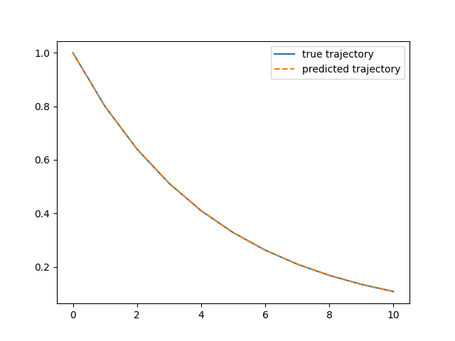
Comparison between ground truth and learned trajectory after training.

Full Code

# helper functions

def zero_1d_array(len: ℝ): ℝ[m]:
    results: ℝ[len] = for i: ℕ(len) -> i*0
    return results

def get_1d_array_length(x: ℝ[m]): ℝ:
    total: ℝ = 0
    temp: ℝ = 0
    for i:
        temp = x[i]
        total += 1
    return total

def append(x: ℝ[m], var: ℝ): ℝ[n]:
    new_length: ℝ = get_1d_array_length(x) + 1
    results: ℝ[new_length] = zero_1d_array(new_length)
    for i:ℕ(new_length):
        if i<get_1d_array_length(x):
            results[i] = x[i]
        else:
            results[i] = var
    return results

# training code
# dy/dt = -θy
# here, θ is a parameter to learn

def f(y: ℝ, θ: ℝ): ℝ:
    return -θ * y

timesteps: ℕ = 10
dt: R = 0.1

def solver(θ: ℝ): ℝ[m]:
   y: ℝ = 1.0
   y_array: ℝ[1] = [1.0]
   for i:ℕ(timesteps):
       dy = f(y, θ)
       y += dt * dy
       y_array = append(y_array, y)
   return y_array

true_theta: ℝ = 2.0
y_true: ℝ[m] = solver(true_theta)

def calculate_loss(θ: ℝ): ℝ:
    y_predicted: ℝ[n] = solver(θ)
    L: ℝ = 0.0
    m: ℝ = get_1d_array_length(y_predicted)
    for i:ℕ(m):
        L += (y_predicted[i] - y_true[i]) ** 2
    return L/m

θ: ℝ = 1.0
learning_rate: ℝ = 0.1
epochs: ℝ = 1000

for i:ℕ(epochs):
    g = grad(calculate_loss, θ)
    θ = θ - learning_rate * g

y_predicted: ℝ[m] = solver(θ)
plot_trajectories(y_true, y_predicted)