Physika Language Reference

Physika programs are stored in .phyk files. Physika uses Unicode math symbols for type annotations and compiles to PyTorch via a parser built with PLY.

Types

ℝ Real number

x : ℝ = 3.14

ℤ Integer

x : ℤ = 3

ℂ Complex

x : ℂ = 3 + 1j

1-D array

v : ℝ[6] = [1, 2, 3.0, 5, 6, 7.0]
u : ℤ[2] = [2, 4, 1, 6, 3, 5]

2-D array (matrix)

A : ℝ[3, 3] = [[1, 0, 0], [0, 1, 0], [0, 0, 1]]

Symbol

x, y: Symbol

Symbolic Function

u: Function

Declarations and Expressions

Variables are declared with a type annotation:

x : ℝ = [1.0, 2.0, 3.0, 5.0, 6.0, 7.0]
y : ℝ[3] = x[0:2] + x[0:2]
z : ℝ[3] = y + [1, 3, 4]

Printing a bare variable name outputs its value at runtime:

x
y
z

Output:

[1.0, 2.0, 3.0, 5.0, 6.0, 7.0] ∈ ℝ[6]
[2.0, 4.0, 6.0] ∈ ℝ[3]
[3.0, 7.0, 10.0] ∈ ℝ[3]

Functions

def f(x : ℝ): ℝ:
    return x * x

f(3)

Output:

9.0 ∈ ℝ

Symbolic expression

x, y: Symbol
f = x**2 + y**2
f

Output:

x**2.0 + y**2.0 ∈ Add

Symbolic Function call

x, y: Symbol
u: Function
u(x, y)

Output:

u(x, y) ∈ u

Control Flow Operators

Conditionals

x : ℝ = 0.3
if x > 0.5:
   y = 3 * (x - 0.75)**2
else:
   y = x**2 + 2

y

Output:

2.09 ∈ ℝ

Output:

2.0 ∈ ℝ

Gradients

def f(x: ℝ): ℝ:
 if x > 0.0:
     return x * x
 else:
     return - x

# positive bracnh
a : ℝ = 3
f(a)
grad(f(a), a)

Output:

9.0 ∈ ℝ
6.0 ∈ ℝ

# negative branch
b : ℝ = - 2
f(b)
grad(f(b), b)

Output:

2.0 ∈ ℝ
-1.0 ∈ ℝ

grad calls compute_grad from the runtime, which differentiates f with respect to its argument using torch.autograd.grad.

Differentiable For Loops

The four loop forms in Physika are differentiable. grad() computes a gradient using Pytorch’s autograd.

For-expression

for i : ℕ(n) → expr constructs an array using torch.stack([...]), which is differentiable:

def scale_vec(x : ℝ): ℝ[3]:
    return for i : ℕ(3) → x * (i + 1)

s : ℝ = 2
scale_vec(s)
grad(scale_vec(s), s)

Output:

[2.0, 4.0, 6.0] ∈ ℝ[3]
[1.0, 2.0, 3.0] ∈ ℝ[3]

The gradient [1, 2, 3] is the Jacobian d(scale_vec)/ds.

Implicit range for-loop

def dot_with_arr(s : ℝ): ℝ:
    a : ℝ[4] = [1, 2, 3, 4]
    result : ℝ = 0
    for i:
        result += s * a[i]
    return result

s : ℝ = 1
grad(dot_with_arr(s), s)

Output:

10.0 ∈ ℝ

Multi-index loop (for i j k:)

Multi-index accumulation loops compile to torch.stack / torch.sum and are fully differentiable:

def matmul_scale(s : ℝ): ℝ:
    A : ℝ[2, 2] = [[1.0, 2.0], [3.0, 4.0]]
    I : ℝ[2, 2] = [[1.0, 0.0], [0.0, 1.0]]
    C : ℝ[2, 2]
    for i j k:
        C[i, j] += s * A[i, k] * I[k, j]
    return sum(C)

s : ℝ = 1.0
grad(matmul_scale(s), s)

Output:

10.0 ∈ ℝ

Jacobian of vector output functions

When the function returns a vector or tensor, grad() returns the full Jacobian matrix instead of a gradient vector:

# f: ℝ → ℝ[n]
# grad() returns a vector (df[i]/ds)
def cos_freqs(x : ℝ): ℝ[4]:
    return for i : ℕ(4) → cos(x * (i + 1.0))

grad(cos_freqs(x), x)
# [-sin(x), -2sin(2x), -3sin(3x), -4sin(4x)]

# f: ℝ[n] → ℝ[n]
# calling grad() for f with relation to x returns a matrix (df[i]/dx[j])
def elementwise_sq(x : ℝ[n]): ℝ[n]:
    return for i → x[i] ** 2

ev : ℝ[3] = [1.0, 2.0, 3.0]
grad(elementwise_sq(ev), ev)

Output:

[[2.0, 0.0, 0.0], [0.0, 4.0, 0.0], [0.0, 0.0, 6.0]] ∈ ℝ[3,3]

Type Checker

Physika’s type checker runs Hindley-Milner type inference over a given program before execution and validates scalars (ℝ, ℕ, ℂ) , string values, arrays and matrices shape compatibility for indexing, slicing, and element-wise operations. It also checks that function calls and return values match their declared types.

Errors are reported with the source line number or the enclosing function/class name where the mismatch was detected.

Type Representations

Every expression is assigned one of these types:

TScalar — A scalar ground type: ℝ, ℕ, ℂ, or string.
TVar — An unknown type variable used during unification, (α0, α1, etc).
TDim — An unknown dimension resolved at unification step (δ0, δ1, etc).
TTensor — A tensor type ℝ[d0, d1, ...] whose dimensions are one of:
- int — A concrete size from a literal annotation (ℝ[5]).
- str — A symbolic size from a generic parameter (ℝ[n]).
- TDim - For an unknown dimension (ℝ[δ0]).
TFunc — A function type (p0, p1, ...) → ret, where pN refers to parameters types and ret refers to the return type.
TInstance — the type of a class value (instance(FullyConnectedNet)).

`VarCounter` class

Generates unique placeholder names when running a Physika program which are resolved at unification step.

VarCounter:
- new_var() → TVar("α0"), TVar("α1"), etc   (unknown type)
- new_dim() → TDim("δ0"), TDim("δ1"), etc  (unknown dimension)
- reset()   → restart from 0, called by run() at session start.

Both new_var and new_dim draw from the same counter so α2 and δ2 can never both exist simultaneously.

`Substitution` class

A dictionary {name: Type} that records types resolved at unification step. Substitution starts empty at the beginning of each function, class, and statement checkers and grows as unify discovers equalities between type variables and concrete types.

Substitution support three methods:

apply(t):
Resolve an unknown variable type TVar and replace every bound variable with its value. Unbound variables are returned unchanged. Following chains: α1 → α0 → ℝ

apply_dim(d):
Same as apply but for a single tensor dimension entry (TDim, TVar, or a TScalar).

compose(other:Substitution):
Merge two substitutions. Apply self to every value in other, then include self’s own bindings.

Errors include the source line number where the mismatch was detected.

Unification

The unification step determines whether two types can be made equal and finding a substitution (Substitution) that records the bindings to do so.

Unification step is needed at every point where two types must agree, which is present in three main places of type checker algorithm:

Expression inference (infer_expr), when:
- Inferring the type of arithmetic operations, both operand types are unified so that tensor shapes must match.
- Inferring the types of an array. All element types are inferred first into a list. Then the first element’s type is used as a base, and each subsequent element’s type is unified against it.
- Calling a user-defined function or class, each argument type is unified against the declared parameter type.
Statement inference (infer_stmts), when:
- Checking a declaration (a : ℕ = 1). The declared type is unified against the inferred type of the right-hand side.
- Verifying a return statement. The inferred return type is unified against the function’s declared return type.
- Checking an if/else statement, the types of the two branches are unified with each other and with the declared return type. Hoisting variables from if/else branches has its two inferred types unified so the outer scope gets a single type.
Top-level checkers (check_function, check_class, check_statement), when:
- Running infer_stmts over a function or class body, the declared return type is unified against the final body expression type.
- At program level, running check_statement unifies the declared type of a decl node against the inferred type of its right-hand side.

unify(t1, t2, s) resolves both types through the current substitution s, checking for:

Equal types: Returns s unchanged.
Type variable (TVar) on either side: Binds the variable to the other type and extends s. An occurs check prevents infinite types (e.g. α0 = ℝ[α0]).
Two scalars: raises TypeError if they differ (e.g. ℝ ≠ ℂ), and if subset (ℕ ⊂ ℝ), s is unchanged.
Two tensors: Must have the same rank. Each dimension pair is unified with unify_dim.
Two functions: Must have the same number of parameters. Each parameter type is unified, then the return types are unified.
Two instances: raises TypeError if the class names differ.

Dimension entries may be concrete integers (3), symbolic strings ("n"), or unresolved type variables (TDim). unify_dim(d1, d2, s) resolve dimension types through s, binding a variable if one side is unknown, and raises TypeError when two concrete values differ.

Expression type inference

Physika expression forms (numeric literals, variables, imaginary unit, arrays, indexing, arithmetic operators, function calls, for-expressions, etc) are handled by a dedicated expr_* function in physika/utils/infer_expr.py.

Every handler receives an ExprContext that bundles the four environment arguments (env, s, func_env, class_env):

env: Maps variable names to their current Type.
s: Substitution accumulated so far. Bindings from sub-expressions are visible to later ones.
func_env: Maps function names to (param_types, return_type).
class_env: Maps class names to their definition dicts.

Each handler returns (inferred_type, updated_substitution).

infer_expr (Top-level dispatcher)

Handles four cases before dispatching on node[0] via EXPR_DISPATCH:

None input: (None, s) with no error.
Bare int or float: (ℝ, s).
Any other non-tuple: (None, s) with no error.
Unknown tag: add_error("Unknown expression type: <tag>") + (None, s)

Then, each expression type in an ASTNode is dispatched to infer the type. The substitution s is threaded through every recursive call so that unification bindings made by sub-expressions are visible to the next ones.

expr_num (Numeric literal ("num", value))

Always returns ℝ regardless of value. No environment lookup needed:

expr_num(("num", 3.14), ctx)  →  (ℝ, s)

expr_imaginary (Imaginary unit ("imaginary",))

Returns ℂ at the top level, but ℝ when "i" appears in env as a for-expression loop variable that shadows the imaginary unit:

expr_imaginary(("imaginary",), ctx)           →  (ℂ, s)
expr_imaginary(("imaginary",), ctx_with_i=ℝ)  →  (ℝ, s)

expr_var (Variable reference ("var", name))

Looks up name in env and applies pending substitutions. Returns (None, s) when the variable is not in scope:

# env = {"x": ℝ[3]}
expr_var(("var", "x"), ctx)   →  (ℝ[3], s)
expr_var(("var", "y"), ctx)   →  (None, s)   # not in scope

expr_array (Array literal ("array", [e0, e1, ...]))

Infers each element’s type, unifies them pairwise to find a common element type, and returns ℝ[n] where n is the number of elements. Inconsistent element types are reported via add_error. When a TVar element is unified against a concrete type, the binding is written into the returned substitution:

expr_array(("array", [num(1), num(2), num(3)]), ctx)    →  (ℝ[3], s)
expr_array(("array", []), ctx)                          →  (ℝ[0], s)
# nested [[1,2],[3,4]]
expr_array(("array", [arr([1,2]), arr([3,4])]), ctx)    →  (ℝ[2,2], s)
# env = {"x": α0}  →  unify(α0, ℝ) writes α0→ℝ
expr_array(("array", [("var","x"), ("num",1.0)]), ctx)  →  (ℝ[2], s{α0→ℝ})

expr_index (1D subscript ("index", arr_name, idx_expr))

Peels the leading dimension of arr_name. A 1D array returns ℝ and a a higher-rank array returns the remaining dims as a tensor. When the index expression has type TDim or TVar, unify_dim is called against the leading dimension, which may bind that variable (depending on Substitution context):

# v : ℝ[5]
expr_index(("index","v",("num",2)), ctx)    →  (ℝ, s)
# v : ℝ[5],  i : δ0  →  unify_dim(δ0, 5, s) binds δ0→5
expr_index(("index","v",("var","i")), ctx)  →  (ℝ, s{δ0→5})
# A : ℝ[3,4]  →  select a row (vector)
expr_index(("index","A",("num",0)), ctx)    →  (ℝ[4], s)

Errors:

unknown variable → (None, s)
indexing a scalar → add_error.

expr_indexN (ND subscript ("indexN", arr_name, [i0, i1, ...]))

Generalises expr_index to an arbitrary number of indices, each unified against the corresponding leading dimension. Returns ℝ for a full index, a lower-rank tensor for partial indexing, or (None, s) with an error for over-indexing:

# T : ℝ[2,3,4]
expr_indexN(("indexN","T",[num(0),num(1),num(2)]), ctx)  →  (ℝ, s)        # full
expr_indexN(("indexN","T",[num(0)]),               ctx)  →  (ℝ[3,4], s)   # partial
# 4 indices on rank-3 tensor
expr_indexN(("indexN","T",[num(0)]*4), ctx)              →  (None, s) + "Over-indexed 'T': 4 indices for a rank-3 tensor"

expr_chain_index (Chained subscript ("chain_index", inner_expr))

Infers inner_expr first, then peels one more leading dimension from the result:

# A : ℝ[3,4]  →  A[0][k] → ℝ
expr_chain_index(("chain_index", ("index","A",num(0))), ctx)  →  (ℝ, s)
# T : ℝ[2,3,4]  →  T[0][1] → ℝ[4]
expr_chain_index(("chain_index", ("index","T",num(0))), ctx)  →  (ℝ[4], s)
# v : ℝ[2]  →  v[0][k] is over-indexing
expr_chain_index(("chain_index", ("index","v",num(0))), ctx)  →  (None, s) + "Chain index applied to a scalar"

expr_slice (Slice ("slice", arr_name, start_expr, end_expr))

Slices the leading dimension of arr_name. Trailing dimensions of higher-rank arrays are preserved unchanged.

Literal bounds Length computed statically:

# v : ℝ[6]
expr_slice(("slice","v",num(1),num(4)), ctx)  →  (ℝ[3], s)
# A : ℝ[3,4]
expr_slice(("slice","A",num(0),num(2)), ctx)  →  (ℝ[2,4], s)

Static semantic errors reported when both bounds are literals:

Negative start or end.
end < start (inverted range).
end == start (empty slice).
start ≥ leading_dim (start out of bounds).
end > leading_dim (end out of bounds).

Dynamic bounds When either bound is a non-literal (a loop variable), a fresh TDim("δN") replaces the sliced leading dimension so rank and trailing dims are still preserved:

# v : ℝ[6],  i : ℝ  (value unknown at compile time)
expr_slice(("slice","v",("var","i"),num(4)), ctx)  →  (ℝ[δ0], s)
# A : ℝ[3,4],  i : ℝ
expr_slice(("slice","A",("var","i"),num(2)), ctx)  →  (ℝ[δ0,4], s)

The TDim placeholder stays unresolved until bound information (e.g. from a loop binder that knows i ∈ [0, n)) is propagated.

expr_add_sub (Addition / subtraction ("add" or "sub", left, right))

Infers both operands (threading the substitution left-to-right) and unifies their shapes. Broadcasting rules:

Tensor + Tensor → shapes must match. Mismatch calls add_error.
Tensor + Scalar (either order) → tensor shape returned.

Scalar + Scalar → ℝ:

# x : ℝ[3],  y : ℝ[3]
expr_add_sub(("add",("var","x"),("var","y")), ctx)   →  (ℝ[3], s)
# x : ℝ[3],  scalar 1.0  (broadcast)
expr_add_sub(("add",("var","x"),("num",1.0)), ctx)   →  (ℝ[3], s)
# x : ℝ[3],  y : ℝ[5]  →  shape mismatch error
expr_add_sub(("add",("var","x"),("var","y")), ctx)   →  (None, s) + "Shape mismatch in add: ℝ[3] vs ℝ[5]"

expr_mul (Multiplication ("mul", left, right))

Infers both operands and unifies shapes for tensor operands. Broadcasting rules same as expr_add_sub:

Tensor × Tensor: shapes must match, a mismatch calls add_error.
Tensor × Scalar (either order): tensor shape returned.

Scalar × Scalar: ℝ:

# x : ℝ[3]
# x * 2
expr_mul(("mul",(TTensor(((3, "invariant"),))),("num",2.0)), ctx) → (ℝ[3], s)
# 2 * 3
expr_mul(("mul",("num",2.0),("num",3.0)), ctx) → (ℝ, s)
# x : ℝ[3] * y : ℝ[5]
# shape mismatch error
expr_mul(("mul",("var","x"),("var","y")), ctx) → (None, s) + "Shape mismatch in mul: ℝ[3] vs ℝ[5]"

expr_div (Division ("div", numerator, denominator))

Tensor / Scalar: result has the shape of the numerator.
Scalar / Scalar: ℝ.

Tensor / Tensor: shapes must match for elementwise division. A mismatch calls add_error:

# x : ℝ[3]
# x / 2
expr_div(("div",(TTensor(((3, "invariant"),))),("num",2.0)), ctx)  → (ℝ[3], s)

# 6 / 2
expr_div(("div",("num",6.0),("num",2.0)), ctx) → (ℝ, s)

# x : ℝ[3]
# y : ℝ[3]
expr_div(("div",(TTensor(((3, "invariant"),))),(TTensor(((3, "invariant"),)))), ctx) → (ℝ[3], s)

# x : ℝ[3]
# z : ℝ[2]
# shape mismatch error
expr_div(("div",(TTensor(((3, "invariant"),))),(TTensor(((2, "invariant"),)))), ctx) → (None, s) + "Shape mismatch in div: ℝ[3] vs ℝ[2]"

expr_matmul (Matrix multiplication ("matmul", left, right))

Inner dimensions must match. Supported rank combinations:

Vector @ Vector (same length) → scalar ℝ (dot product).
Matrix @ Matrix (ℝ[m,n] @ ℝ[n,p]) → ℝ[m,p]. (And so on for higher ranks)

Incompatible shapes calls add_error:

# A : ℝ[2,3],  B : ℝ[3,4]
expr_matmul(("matmul",("var","A"),("var","B")), ctx) → (ℝ[2,4], s)
# u : ℝ[3],  v : ℝ[3]  →  dot product
expr_matmul(("matmul",("var","u"),("var","v")), ctx) → (ℝ, s)

expr_pow (Exponentiation ("pow", base, exponent))

The result has the same type as the base. The exponent is inferred and it should not affect the output shape:

# x : ℝ[3]
# x ** 2
expr_pow(("pow",("var","x"),("num",2.0)), ctx) → (ℝ[3], s)
# x ** 3
expr_pow(("pow",("num",2.0),("num",3.0)), ctx) → (ℝ, s)

expr_neg (Negation ("neg", operand))

The result type equals the operand type:

# x : ℝ[3]
# -x
expr_neg(("neg",("var","x")), ctx) → (ℝ[3], s)
#-1
expr_neg(("neg",("num",1.0)), ctx) → (ℝ, s)

expr_call (Function call ("call", func_name, arg_list))

Resolution order:

Built-in elementwise (exp, sin, cos, sqrt, abs, tanh, log, real, imag): preserve the shape of their first argument.
Built-in reduction (sum): ℝ.
grad(f, x): same type as x.
User-defined functions in func_env: each argument is unified against its declared parameter type and the declared return type is returned. The number of arguments received and declared are also checked.
Unknown call target returns (None, s).

# x : ℝ[3]
expr_call(("call","sin",[("var","x")]), ctx) → (ℝ[3], s)
expr_call(("call","sum",[("var","x")]), ctx) → (ℝ, s)
expr_call(("call","grad",[("num",1.0),("var","x")]), ctx) → (ℝ[3], s)
# func_env = {"f": ([ℝ[3]], ℝ[3])}
expr_call(("call","f",[("var","x")]), ctx) → (ℝ[3], s)

expr_for_expr (For-expression ("for_expr", loop_var, size_expr, body_expr))

Loop variable is bound as ℕ inside the body. The outer size is prepended as the leading tensor dimension:

Scalar body is inferred to type ℝ[n].
Tensor body ℝ[d0, d1, ...] is inferred to ℝ[n, d0, d1, ...].

Fresh TDim placeholder used instead of n for non-literal expressions:

# body = i (ℕ, resolved as ℝ for scalar context)
expr_for_expr(("for_expr","i",("num",3.0),("imaginary",)), ctx, new_dim) → (ℝ[3], s)

# body = [1.0, 2.0] (ℝ[2]) — outer size 4 prepended
expr_for_expr(("for_expr","i",("num",4.0),("array",[num(1),num(2)])), ctx, new_dim) → (ℝ[4,2], s)

# nested: inner for produces ℝ[4], outer for prepends 3 → ℝ[3,4]
expr_for_expr(("for_expr","i",("num",3.0), inner_for_expr_node), ctx, new_dim) → (ℝ[3,4], s)

expr_for_expr_range (Range for-expression ("for_expr_range", loop_var, start_expr, end_expr, body_expr))

Like expr_for_expr but the outer size is computed as end − start from explicit bounds. When either bound is non-literal a fresh TDim is introduced instead:

Both bounds literal: outer dimension = int(end) − int(start).

Either bound dynamic: outer dimension = fresh TDim:

# range ℕ(0, 4) (4 elements), scalar body
expr_for_expr_range(("for_expr_range","i",("num",0.0),("num",4.0),("imaginary",)), ctx, new_dim) → (ℝ[4], s)

# range ℕ(0, 2) (2 elements), body ℝ[3]
expr_for_expr_range(("for_expr_range","i",("num",0.0),("num",2.0), body), ctx, new_dim) → (ℝ[2,3], s)

# dynamic end bound (ℕ(0, n))
expr_for_expr_range(("for_expr_range","i",("num",0.0),("var","n"),("imaginary",)), ctx, new_dim) → (ℝ[δ0], s)

expr_cond (Comparison condition ("cond_op", left, right))

Handles six comparison operators: cond_eq (==), cond_neq (!=), cond_lt (<), cond_gt (>), cond_leq (<=), cond_geq (>=).

Both operands are inferred and their resolved types are unified (type error reported if unification fails). The return type is the inferred left operand type. If this is None the right operand type is used. Finally, if both are None the fallback is ℝ:

# x : ℝ
# y : ℝ
expr_cond(("cond_gt", ("var","x"), ("var","y")), ctx)   →  (ℝ, s)

# u : ℝ[3]
# v : ℝ[3]
expr_cond(("cond_eq", ("var","u"), ("var","v")), ctx)   →  (ℝ[3], s)

# x : ℝ
# v : ℝ[3]
# type mismatch and left type returned
expr_cond(("cond_lt", ("var","x"), ("var","v")), ctx)   →  (ℝ, s) + "ℝ is not comparable with ℝ[3] at 'cond_lt' expression"

Statement type inference

Physika statement type inference at function’s body and top-level programs (declaration, assigments, for-loops, if-else blocks, random sampling, etc) are handled by a handler stmt_* function in physika/utils/infer_stmts.py.

Every handler receives an StmtContext that bundles six environment arguments (env, s, func_env, class_env, func_name, return_type):

env: Maps variable names to their current Type.
s: Substitution accumulated so far. Bindings from sub-expressions are visible to later ones.
func_env: Maps function names to (param_types, return_type).
class_env: Maps class names to their definition dicts.
func_name: User defined function name. Used when calling check_function from main type checking algorithm.
return_type: Used especifically in body_if_return and body_if_else_return to unify the return expression type against it.

Each handler unifies inferred type against declared type. If a mismatch is found, an error is reported. stmt_* handlers instead of returning the inferred type, updates ctx: StmtContext with inferred and declared information. Physika support statements as follows.

1. At function level (body_statements).

stmt_body_decl (("body_decl", var_name, var_type, expr))

Typed variable declaration inside a function body (x : ℝ = expr). Infers the type of expr, unifies it against the declared type, and registers the resolved type in env. On mismatch the inferred type is stored so inference can continue.

Match: env[var_name] is set to the declared type:

# x : ℝ = 3.14
stmt_body_decl(("body_decl","x","ℝ",("num",3.14)), ctx)
# ctx.env["x"] == ℝ

Mismatch: error reported, env[var_name] is set to the inferred type:

# v : ℝ[3] = 2.0
stmt_body_decl(("body_decl","v",("tensor",[(3,"invariant")]), ("num",2.0)), ctx)
# errors == ["In 'f': 'v' declared ℝ[3], inferred ℝ: Cannot unify tensor ℝ[3] with scalar ℝ"]
# inferred type stored so inference continues
# ctx.env["v"] == ℝ

stmt_body_assign (("body_assign", var_name, expr))

Untyped assignment inside a function body (x = expr). Infers the type of expr and registers it in env. There is no declared type to check against so no error is emitted. If inference returns None a fresh type variable is stored.

Scalar:

# x = 3.0
stmt_body_assign(("body_assign","x",("num",3.0)), ctx)
# ctx.env["x"] == ℝ,  errors == []

Array:

# v = [1.0, 2.0, 3.0]
stmt_body_assign(("body_assign","v",
                  ("array",[num(1),num(2),num(3)])), ctx)
# ctx.env["v"] == ℝ[3]

If unknown type, a fresh type variable (TVar) stored:

# x not in env
stmt_body_assign(("body_assign","x",("var","unknown")), ctx)
# ctx.env["x"] == TVar("α0")

stmt_body_if_return (("body_if_return", cond_expr, ret_expr))

if return statement inside a function body:

def f(x: ℝ): ℝ:
    if x > 0.0:
        return x * x

The declared return type is unified against the inferred type and a mismatch calls add_error:

# declared return type: ℝ
stmt_body_if_return(("body_if_return", cond, ("var","x")), ctx)

# ctx.return_type = ℝ,
#  v : ℝ[3]
stmt_body_if_return(("body_if_return", cond, ("var","v")), ctx)
# errors → "if-return type mismatch: declared ℝ, got ℝ[3]"

stmt_body_if_else_return (("body_if_else_return", cond_expr, then_expr, else_expr))

if/else return statement inside a function body:

def f(x: ℝ): ℝ:
    if x > 0.0:
        return x * x
    else:
        return -x

Type inference checks for then_expr and else_expr types, which are unified against each other. A mismatch here means the two branches disagree on what the function returns. Both errors are independent. Then the unified branch (with the inferred type) is unified with the declared type:

# ctx.return_type = ℝ,
# x : ℝ
stmt_body_if_else_return(("body_if_else_return", cond, ("var","x"), ("num",0.0)), ctx)

# ctx.return_type = ℝ
# v : ℝ[3]
stmt_body_if_else_return(("body_if_else_return", cond, ("var","v"), ("num",0.0)), ctx)
# Two errors:
# "if/else branch type mismatch: then=ℝ[3], else=ℝ: ..."
# "if/else return type mismatch: declared ℝ, got ℝ[3]: ..."

stmt_body_if_else (("body_if_else", cond_expr, then_stmts, else_stmts) / ("body_if", cond_expr, then_stmts))

if/else and if-only node inside a function body where neither branch ends with return. Both branch bodies are run through infer_stmts so that type errors inside them are caught:

def f(x: ℝ): ℝ:
    if x > 0.0:
        y : ℝ = x * x
    else:
        y : ℝ = 0.0 - x

Error inside a branch are tracked:

def f(x: ℝ): ℝ:
    if x > 0.0:
        v : ℝ[3] = 2.0
# declared ℝ[3] but inferred ℝ
# type checker call:
stmt_body_if_else(("body_if_else", cond,
                   [("body_decl","v",("tensor",[(3,"invariant")]),("num",2.0))],
                   []), ctx)
# "In 'f': 'v' declared ℝ[3], inferred ℝ"

2. Inside function and for loop bodies.

stmt_body_for (("body_for", loop_var, loop_body, indexed_arrays))

Inference statements for for-loop (for i:) inside a function body. Registers loop_var as T_NAT, then runs infer_stmts over the body. New bindings from the body are added to ctx.env.

The fourth element indexed_arrays is to infer the size of the array to range over using range(len(arr)) and type inference ignores this argument. In a physika program the body must index an array:

# for i:
#     total = arr[i]
stmt_body_for(("body_for","i",
               [("loop_assign","total",("index","arr",("var","i")))],
               ["arr"]), ctx)
# ctx.env["i"] == ℕ
# ctx.env["total"] == ℝ

stmt_body_for_range (("body_for_range", loop_var, start, stop, loop_body))

Ranged for loop (for i : ℕ(n):). Similar syntax as previous loops but here, an user can explicitly define the values to range over. In the type checker, the start and stop expressions are not checked. Our type system check the body statements:

# for i : ℕ(10):
#     acc = x
stmt_body_for_range(("body_for_range","i",("num",0),("num",10),
                     [("loop_assign","acc",("var","x"))]), ctx)
# ctx.env["i"] == ℕ
# ctx.env["acc"] == ℝ

stmt_body_zeros_decl (("body_zeros_decl", var_name, type_spec))

Zero initialised array declaration (C : ℝ[n, o]). Registers the declared type in env so that a subsequent for i j k: accumulation loop can look up C’s shape for index unification:

# C : ℝ[3, 4]
stmt_body_zeros_decl(("body_zeros_decl","C",
                       ("tensor",[(3,"invariant"),(4,"invariant")])), ctx)
# ctx.env["C"] == ℝ[3,4]

If the type cannot be resolved, a fresh TVar is added.

stmt_body_for_accum (("body_for_accum", loop_vars, loop_body))

Multi-variable accumulation loop (for i j k:). Each loop variable is registered as a fresh TDim (dimension unification variable).``TDim`` is required because each variable is later unified against a specific array dimension:

# for i j k:
#     C[i, j] += A[i, k] * B[k, j]
stmt_body_for_accum(("body_for_accum",["i","j","k"],[...]), ctx)
# ctx.env["i"], ["j"], ["k"]  are all fresh TDim instances

stmt_for_assign (("loop_assign", var_name, rhs))

Assignment statement inside a for loop body (y = expr). Infers the type of rhs and registers it in env. If inference returns None a fresh TVar is stored and type checking continues, allowing for unification:

# y = arr[i]
stmt_for_assign(("loop_assign","y",("index","arr",("var","i"))), ctx)
# ctx.env["y"] == ℝ

stmt_for_pluseq (("for_pluseq", arr_name, idx_exprs, rhs) / ("loop_index_pluseq", arr_name, idx_exprs, rhs))

In place accumulation (+=) inside a for loop body. Two forms:

"for_pluseq": scalar accumulation (total += expr). Only the RHS is inferred and no need for index unification.
"loop_index_pluseq": indexed accumulation (C[i, j] += expr). Each index expression is unified against the matching dimension of the target array in ctx.s, binding the TDim loop variables to concrete sizes.

Indexed form: C : ℝ[3,4], i and j are TDim loop vars:

stmt_for_pluseq(("loop_index_pluseq","C",
                 [("var","i"),("var","j")],("num",1.0)), ctx)
# ctx.s: binds i TDim to 3 and j TDim to 4
# ctx.env["i"], ctx.env["j"]: hold the original TDim objects

stmt_loop_if (("loop_if", cond_expr, then_body))

if conditional inside a for loop body:

def f(x: ℝ): ℝ:
   for i:
      if arr[i] > 0.0:
         pos = pos + arr[i]

Infers cond_expr and runs infer_stmts over then_body. New bindings from the body are added to ctx.env:

stmt_loop_if(("loop_if", cond,
              [("loop_assign","result",("var","x"))]), ctx)
# ctx.env["result"] == ℝ

stmt_loop_if_else (("loop_if_else", cond_expr, then_body, else_body))

Similar to stmt_loop_if, but includes the else branch statements infernece:

def f(x: ℝ): ℝ:
   for i:
      if arr[i] > 0.0:
         pos = pos + arr[i]
      else:
         neg = neg + arr[i]

Infers cond_expr and runs infer_stmts over both branches. New bindings from each branch are added to ctx.env:

stmt_loop_if_else(("loop_if_else", cond,
                   [("loop_assign","a",("var","x"))],
                   [("loop_assign","b",("num",0.0))]), ctx)
# ctx.env["a"] == ℝ
# ctx.env["b"] == ℝ

stmt_decl (("decl", var, type_spec, expr))

Handles program-level variable declarations which includes type annotation. The expression type is inferred and unified against the declared type:
```
a : ℝ = 4.0
# AST: ("decl", "a", "ℝ", ("num", 4.0))
# after: ctx.env["a"] == ℝ
```
stmt_assign (("assign", var, expr))

Since there is no type annotation, the inferred type is stored directly in ctx.env. If the expression type cannot be resolved, a fresh type variable is stored so that later statements can still be checked:
```
a = a + 1.0
# AST: ("assign", "a", ("add", ("var", "a"), ("num", 1.0)))
# after: ctx.env["a"] == ℝ
```
stmt_expr (("expr", expr))

Infers standalone expression statements whose result is not bound to any variable. The expression is type checked so that shape or call-signature errors are caught, but the result is discarded and ctx.env is not modified:
```
f(x)
# AST: ("expr", ("call", "f", [("var", "x")]))
# ctx.env is unchanged; type errors in the call are still reported
```

3. Central dispatcher.

infer_stmts (infer_stmts(stmts, env, s, func_env, class_env, add_error))

Dispatches a list of statement AST nodes to their stmt_* handler functions via STMT_DISPATCH. Called from the main type checking algorithm for both function bodies and top-level programs.

Creates a fresh StmtContext and iterates over stmts. Each node’s tag is looked up in STMT_DISPATCH. Returns the updated (env, s) pair:

env, s = infer_stmts(
    [("body_decl","x","ℝ",("num",1.0)),
     ("body_assign","y",("var","x"))],
    {}, Substitution(), {}, {}, errors.append)
# env == {"x": ℝ, "y": ℝ},  errors == []

`TypeChecker` class

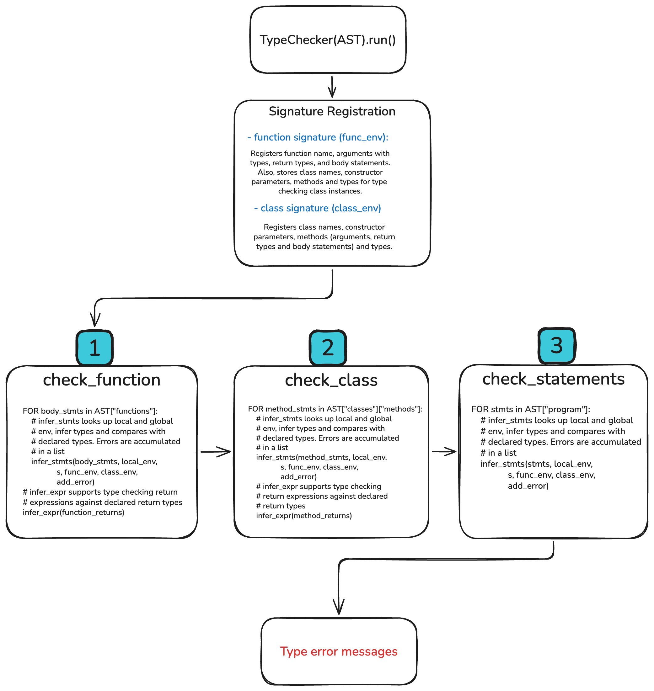
Finally, these components are used to build a type checker system for Physika programs. Physika’s type checker performs three passes over the unified AST:

Signature registration: All function and class signatures are stored in func_env and class_env before any body is examined. Class constructors are stored in func_env as (field_types, TInstance(name)).

Body checking (check_function, check_class): For each def and class, infer_stmts walks statements in order, threading s through every expression to build a local type environment. The return expression is inferred and unified against the declared return type. A mismatch is recorded as an error prefixed with the function or class name.

Program statement checking (check_statement): Top-level stmts nodes are checked in source order. The line number is read from the last element of each statement tuple and prepended to error messages.

Type mismatches are accumulated in self.errors as plain strings.

Below is a figure of Physika’s TypeChecker describing the mentioned workflow:

Symbolic methods

Declare required variables:

x, y : Symbol
u : Function

substitution

f = x**2 + y**2
subs(f, x, 3.0, y, 4.0)

Output:

25.0000000000000 ∈ Float

diff

f = x**3 + 2*(x**2) + x
diff(f, x)

Output:

3*x**2 + 4*x + 1 ∈ Add

lambdify

expr = x**2 + y**2
f = lambdify([x, y], expr)
f(3.0, 4.0)

Output:

25.0 ∈ ℝ

symbolic solve

eq: Equation := 2.0*x + 3.0 = 7.0
symbolic_solve(eq, x)

Output:

[2.00000000000000] ∈ ℝ[1]

Scientific notation

Physika supports scientific notation natively for numeric literals such as 1e5, 2.5e-3 or 6.674e-11.

G: ℝ = 6.674e-11    # gravitational constant (m³·kg⁻¹·s⁻²)
c: ℝ = 3e8          # speed of light (m·s⁻¹)

Greek Letters

Physika supports Greek letters as valid symbols and variables.

Note

Δ (U+0394) is reserved for the Laplacian operator and cannot be used as an identifier.

Uppercase Letters

Symbol	Unicode	Name
Α	U+0391	Alpha
Β	U+0392	Beta
Γ	U+0393	Gamma
Δ	U+0394	Delta (reserved — Laplacian operator)
Ε	U+0395	Epsilon
Ζ	U+0396	Zeta
Η	U+0397	Eta
Θ	U+0398	Theta
Ι	U+0399	Iota
Κ	U+039A	Kappa
Λ	U+039B	Lambda
Μ	U+039C	Mu
Ν	U+039D	Nu
Ξ	U+039E	Xi
Ο	U+039F	Omicron
Π	U+03A0	Pi
Ρ	U+03A1	Rho
Σ	U+03A3	Sigma
Τ	U+03A4	Tau
Υ	U+03A5	Upsilon
Φ	U+03A6	Phi
Χ	U+03A7	Chi
Ψ	U+03A8	Psi
Ω	U+03A9	Omega

Lowercase Letters

Symbol	Unicode	Name
α	U+03B1	alpha
β	U+03B2	beta
γ	U+03B3	gamma
δ	U+03B4	delta
ε	U+03B5	epsilon
ζ	U+03B6	zeta
η	U+03B7	eta
θ	U+03B8	theta
ι	U+03B9	iota
κ	U+03BA	kappa
λ	U+03BB	lambda
μ	U+03BC	mu
ν	U+03BD	nu
ξ	U+03BE	xi
ο	U+03BF	omicron
π	U+03C0	pi
ρ	U+03C1	rho
ς	U+03C2	final sigma
σ	U+03C3	sigma
τ	U+03C4	tau
υ	U+03C5	upsilon
φ	U+03C6	phi
χ	U+03C7	chi
ψ	U+03C8	psi
ω	U+03C9	omega

Import statements

Physika provides module import support to enable code reuse across files.

Import statements are resolved during AST construction. Imported modules are parsed, and only the requested symbols are injected into the current program AST.

# simple import statement
from factorial import fact

fact(1.0)


# import multiple symbols
from diff_functions import f, torch_funcs_with_scalar_R

f(1.0)
torch_funcs_with_scalar_R(1.0)

Physika Language Reference

Types

ℝ Real number

ℤ Integer

ℂ Complex

1-D array

2-D array (matrix)

Symbol

Symbolic Function

Declarations and Expressions

Functions

Symbolic expression

Symbolic Function call

Control Flow Operators

Conditionals

Gradients

Differentiable For Loops

For-expression

Implicit range for-loop

Multi-index loop (for i j k:)

Jacobian of vector output functions

Type Checker

Type Representations

VarCounter class

Substitution class

Unification

Expression type inference

Statement type inference

TypeChecker class

Symbolic methods

substitution

diff

lambdify

symbolic solve

Scientific notation

Greek Letters

Uppercase Letters

Lowercase Letters

Import statements

`VarCounter` class

`Substitution` class

`TypeChecker` class