Parameter Learning for ODE: Lotka-Volterra

In this tutorial we will learn the parameters of the Lotka-Volterra equations — a pair of coupled ODEs that model predator-prey dynamics in ecology. We will use the adjoint method for efficient gradient computation.

The Equations

The Lotka-Volterra system is:

\[ \begin{align}\begin{aligned}\frac{dx}{dt} = \alpha x - \beta xy\\\frac{dy}{dt} = \delta xy - \gamma y\end{aligned}\end{align} \]

Where \(x\) is the prey population, \(y\) is the predator population, and \(\theta = [\alpha, \beta, \gamma, \delta]\) are the parameters we want to learn.

Helper functions

def zero_1d_array(len: ℝ): ℝ[m]:
    results: ℝ[len] = for i: ℕ(len) -> i*0
    return results

def get_1d_array_length(x: ℝ[m]): ℝ:
    total: ℝ = 0
    temp: ℝ = 0
    for i:
        temp = x[i]
        total += 1
    return total

def append(x: ℝ[m], var: ℝ): ℝ[n]:
    new_length: ℝ = len(x) + 1
    results: ℝ[new_length] = zero_1d_array(new_length)
    for i:ℕ(new_length):
        if i<len(x):
            results[i] = x[i]
        else:
            results[i] = var
    return results

Step 1: Define the ODE

def f(state: ℝ[2], θ: ℝ[4]): ℝ:
    x: ℝ = state[0]
    y: ℝ = state[1]
    α: ℝ = θ[0]
    β: ℝ = θ[1]
    γ: ℝ = θ[2]
    δ: ℝ = θ[3]
    dx: ℝ = (α * x) - (β * x * y)
    dy: ℝ = - (γ * y) + (δ * x * y)
    return [dx, dy]

f takes the current state [x, y] and parameters theta and returns the derivatives [dx/dt, dy/dt].

Step 2: Build the RK4 Solver

We use the Runge-Kutta 4 method for higher accuracy than Forward Euler. RK4 evaluates the derivative at four points within each time step:

\[\begin{split}\begin{align*} k_1 &= f(y_n, \theta) \\ k_2 &= f\left(y_n + \frac{h}{2} k_1, \theta\right) \\ k_3 &= f\left(y_n + \frac{h}{2} k_2, \theta\right) \\ k_4 &= f(y_n + h \cdot k_3, \theta) \\ y_{n+1} &= y_n + \frac{h}{6}(k_1 + 2k_2 + 2k_3 + k_4) \end{align*}\end{split}\]

def rk4_step(state: ℝ[2], θ: ℝ[4]): R[2]:
    k1: ℝ[2] = f(state, θ)
    k2_state: ℝ[2] = state + 0.5 * dt * k1
    k2: ℝ[2] = f(k2_state, θ)
    k3_state: ℝ[2] = state + 0.5 * dt * k2
    k3: ℝ[2] = f(k3_state, θ)
    k4_state: ℝ[2] = state + dt * k3
    k4: ℝ[2] = f(k4_state, θ)
    return state + (dt / 6.0) * (k1 + 2.0 * k2 + 2.0 * k3 + k4)

Step 3: Build the Trajectory Solver

We integrate the system forward from initial conditions \(x_0 = 10, y_0 = 1\) over 100 timesteps:

dt: ℝ = 0.1
timesteps: ℝ = 100

def solver(θ: ℝ[4]): ℝ[m]:
    state: ℝ[2] = [10.0, 1.0]
    x_array: ℝ[0] = [10.0]
    y_array: ℝ[0] = [1.0]
    for i:ℕ(timesteps):
        results = rk4_step(state, θ)
        x = results[0]
        y = results[1]
        x_array = append(x_array, x)
        y_array = append(y_array, y)
        state = results
    return [x_array, y_array]

Step 4: Generate Ground Truth Data

We pick true parameters and generate the ground truth trajectories:

true_theta: ℝ[4] = [1.5, 1.0, 3.0, 1.0]
true_results: ℝ[m] = solver(true_theta)
true_x: ℝ[m] = true_results[0]
true_y: ℝ[m] = true_results[1]

Step 5: Adjoint Gradient

To train the Lotka-Volterra ODE model, we use the adjoint state method to compute gradients during optimization. This method is useful because it computes gradients with respect to all parameters using a single backward pass, without storing the full forward trajectory, making it memory-efficient and scalable to long time horizons.

def adjoint_grad(θ: ℝ[4]): ℝ:
    states: ℝ[m] = solver(θ)
    x_array: ℝ[m] = states[0]
    y_array: ℝ[m] = states[1]
    m: ℝ = get_1d_array_length(x_array)
    s: ℝ[2] = [
        2 * (x_array[m-1] - true_x[m-1]),
        2 * (y_array[m-1] - true_y[m-1])
    ]
    L: ℝ[4] = zero_1d_array(4)
    for i:ℕ(m-1):
        idx = m - 1 - i
        x = x_array[idx]
        y = y_array[idx]
        state = [x, y]
        J_state = grad(rk4_step(state, θ), state)
        J_theta = grad(rk4_step(state, θ), θ)
        L += s @ J_theta
        s = s @ J_state
    return L

grad(rk4_step(state, θ), state) differentiates rk4_step with respect to state and grad(rk4_step(state, θ), θ) with respect to theta.

The function adjoint_grad implements the adjoint state method for computing gradients of the Lotka–Volterra ODE parameters.

Forward Pass

The system is defined by discretizing RK4 method for each step using solver(θ) function:

\[y_{n+1} = \mathrm{RK4}(y_n, \theta)\]

Terminal Condition

The adjoint variable is defined as the gradient of the loss with respect to the final state:

\[s_N = \frac{\partial \mathcal{L}}{\partial y_N}\]

The loss function is defined as:

\[\mathcal{L}(\theta) = \| y_N - y_N^{\mathrm{true}} \|^2\]

For the chosen loss:

\[s_N = 2 (y_N - y_N^{\mathrm{true}})\]

Backward Pass

The RK4 step is treated as a function:

\[y_{n+1} = f(y_n, \theta)\]

The Jacobians are calculated as:

State Jacobian:

\[J_{\mathrm{state}} = \frac{\partial f(y_n, \theta)}{\partial y_n}\]

Parameter Jacobian:

\[J_{\theta} = \frac{\partial f(y_n, \theta)}{\partial \theta}\]

The adjoint variable is then updated backward in time, and the parameter gradient is accumulated as:

\[ \begin{align}\begin{aligned}L \mathrel{+}= s \, J_{\theta}\\s \mathrel{=} s \, J_{\mathrm{state}}\end{aligned}\end{align} \]

Step 6: Train with Gradient Descent

We start with an initial guess and run 1000 epochs:

θ: ℝ[4] = [1.0, 0.7, 2.5, 0.7]
learning_rate: ℝ = 0.0005
epochs: ℕ = 2000

for i:ℕ(epochs):
    g = adjoint_grad(θ)
    θ = θ - learning_rate * g

After training, theta should be close to [1.5, 1.0, 3.0, 1.0].

Step 7: Visualize Results

pred_results = solver(θ)
plot_trajectories(true_results, pred_results)

Note

plot_trajectories is not a built-in Physika function. Add the following helper function to physika/runtime.py:

def plot_trajectories(true_results, pred_results):
    import matplotlib.pyplot as plt

    plt.plot(true_results[0, :], color="orange", label="Prey (True)")
    plt.plot(pred_results[0, :], color="orange", linestyle="--", label="Prey (Predicted)")

    plt.plot(true_results[1, :], color="green", label="Predator (True)")
    plt.plot(pred_results[1, :], color="green", linestyle="--", label="Predator (Predicted)")

    plt.xlabel("Time Step")
    plt.ylabel("Population")
    plt.title("Lotka-Volterra: True vs Predicted")
    plt.legend()
    plt.show()

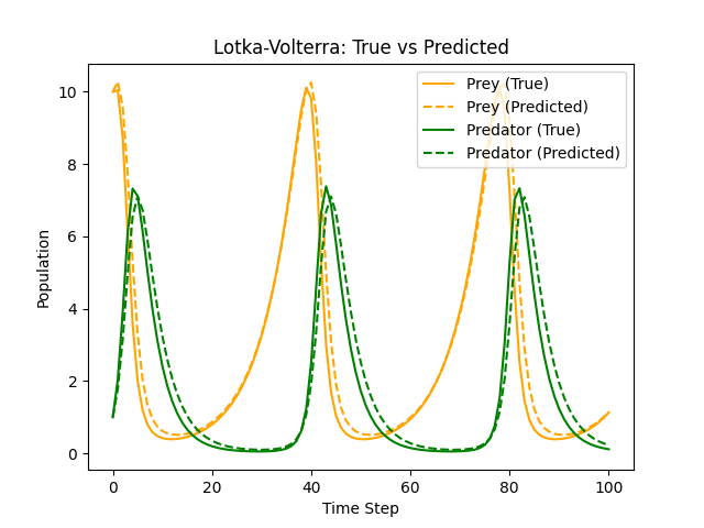
Comparison between ground truth and learned trajectory after training.

Full Code

def zero_1d_array(len: ℝ): ℝ[m]:
    results: ℝ[len] = for i: ℕ(len) -> i*0
    return results

def get_1d_array_length(x: ℝ[m]): ℝ:
    total: ℝ = 0
    temp: ℝ = 0
    for i:
        temp = x[i]
        total += 1
    return total

def append(x: ℝ[m], var: ℝ): ℝ[n]:
    new_length: ℝ = len(x) + 1
    results: ℝ[new_length] = zero_1d_array(new_length)
    for i:ℕ(new_length):
        if i<len(x):
            results[i] = x[i]
        else:
            results[i] = var
    return results

def f(state: ℝ[2], θ: ℝ[4]): ℝ:
    x: ℝ = state[0]
    y: ℝ = state[1]
    α: ℝ = θ[0]
    β: ℝ = θ[1]
    γ: ℝ = θ[2]
    δ: ℝ = θ[3]
    dx: ℝ = (α * x) - (β * x * y)
    dy: ℝ = - (γ * y) + (δ * x * y)
    return [dx, dy]

def rk4_step(state: ℝ[2], θ: ℝ[4]): R[2]:
    k1: ℝ[2] = f(state, θ)
    k2_state: ℝ[2] = state + 0.5 * dt * k1
    k2: ℝ[2] = f(k2_state, θ)
    k3_state: ℝ[2] = state + 0.5 * dt * k2
    k3: ℝ[2] = f(k3_state, θ)
    k4_state: ℝ[2] = state + dt * k3
    k4: ℝ[2] = f(k4_state, θ)
    return state + (dt / 6.0) * (k1 + 2.0 * k2 + 2.0 * k3 + k4)

dt: ℝ = 0.1
timesteps: ℝ = 100

def solver(θ: ℝ[4]): ℝ[m]:
    state: ℝ[2] = [10.0, 1.0]
    x_array: ℝ[0] = [10.0]
    y_array: ℝ[0] = [1.0]
    for i:ℕ(timesteps):
        results = rk4_step(state, θ)
        x = results[0]
        y = results[1]
        x_array = append(x_array, x)
        y_array = append(y_array, y)
        state = results
    return [x_array, y_array]

true_theta: ℝ[4] = [1.5, 1.0, 3.0, 1.0]
true_results: ℝ[m] = solver(true_theta)
true_x: ℝ[m] = true_results[0]
true_y: ℝ[m] = true_results[1]

def adjoint_grad(θ: ℝ[4]): ℝ:
    states: ℝ[m] = solver(θ)
    x_array: ℝ[m] = states[0]
    y_array: ℝ[m] = states[1]
    m: ℝ = get_1d_array_length(x_array)
    s: ℝ[2] = [
        2 * (x_array[m-1] - true_x[m-1]),
        2 * (y_array[m-1] - true_y[m-1])
    ]
    L: ℝ[4] = zero_1d_array(4)
    for i:ℕ(m-1):
        idx = m - 1 - i
        x = x_array[idx]
        y = y_array[idx]
        state = [x, y]
        J_state = grad(rk4_step(state, θ), state)
        J_theta = grad(rk4_step(state, θ), θ)
        L += s @ J_theta
        s = s @ J_state
    return L

θ: ℝ[4] = [1.0, 0.7, 2.5, 0.7]
learning_rate: ℝ = 0.0005
epochs: ℕ = 2000

for i:ℕ(epochs):
    g = adjoint_grad(θ)
    θ = θ - learning_rate * g

pred_results = solver(θ)
plot_trajectories(true_results, pred_results)

References

• Lotka-Volterra equations — Wikipedia

• Adjoint state method for ODE with rk4

• Adjoint Differentiation — MIT OCW